Theory
In large language model reinforcement learning training, there are two ways to incorporate KL divergence constraints: reward shaping and KL loss. The former directly adds KL estimation to the reward value as a new reward $r \leftarrow r - \beta\cdot KL$; the latter puts the KL estimation term in the loss function, computing $\nabla_\theta \operatorname{KL}(\pi_\theta||\pi_{ref})$ for backpropagation.
Schulman (2020) proposed three methods for estimating KL divergence, among which k3 loss is considered a good estimator with both unbiased and low variance properties. DeepSeek’s GRPO algorithm (Guo et al. 2025) adopted this approach:
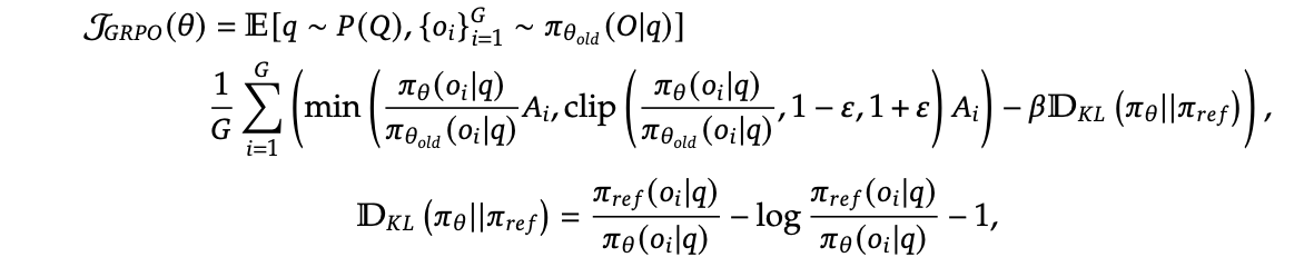
Fig. 1. GRPO Algorithm. (Source: Guo et al. 2025)
However, when using KL Loss, we actually estimate the gradient of KL divergence through sampling, which differs somewhat from Schulman (2020)’s analysis. In training, after constructing the estimator, we directly use it as a loss for backpropagation, hoping it remains a good approximation:
$$ \begin{align*} \nabla_\theta \widehat{\operatorname{KL}}(X) &\approx \nabla_\theta \operatorname{KL}(\pi_\theta||\pi_{\theta_{ref}})=\nabla_\theta \int \pi_\theta(x)\cdot\log\left(\frac{\pi_\theta(x)}{\pi_{ref}(x)}\right)dx\\ &= \int \nabla_\theta\pi_\theta(x)\cdot\log\left(\frac{\pi_\theta(x)}{\pi_{ref}(x)}\right) + \pi_\theta(x)\nabla_\theta\log\pi_\theta(x)dx\\ &=\int \pi_\theta(x)\cdot\nabla_\theta\log\pi_\theta(x)\log\left(\frac{\pi_\theta(x)}{\pi_{ref}(x)}\right) + \pi_\theta(x)\cdot \frac{1}{\pi_\theta(x)}\nabla_\theta\pi_\theta(x)dx\\ &=E_{x\sim\pi_\theta}\left[\nabla_\theta\log\pi_\theta(X)\cdot\log\left(\frac{\pi_\theta(X)}{\pi_{ref}(X)}\right)\right]. \end{align*} $$
However, the gradient of an unbiased KL estimator is not necessarily an unbiased estimator of the KL gradient:
$$ E_{\pi_\theta}[\nabla_\theta \widehat{\operatorname{KL}}(X)] \neq \nabla_\theta E_{\pi_\theta}[ \widehat{\operatorname{KL}}(X)] = \nabla_\theta \operatorname{KL}(\pi_\theta||\pi_{\theta_{ref}}). $$
In fact, they differ by one term:
$$ \begin{align*} \nabla_\theta E_{\pi_\theta}[f_\theta(X)] &= \int \nabla_\theta\pi_\theta(x)\cdot f_\theta(x) + \pi_\theta(x)\cdot\nabla_\theta f_\theta(x) dx\\ &= \int \pi_\theta(x)\cdot\nabla_\theta \log\pi_\theta(x)\cdot f_\theta(x) dx + \int \pi_\theta(x)\cdot\nabla_\theta f_\theta(x) dx\\ &= E_{\pi_\theta}[\nabla_\theta\log\pi_\theta(X)\cdot f_\theta(X)] + E_{\pi_\theta}[\nabla_\theta f_\theta(X)]. \end{align*} $$
For samples $X\sim\pi_\theta(\cdot)$ generated by the policy, taking $\widehat{\operatorname{KL}}$ as k1, k2, and k3 loss respectively:
-
k1
$$ \begin{align*} \widehat{\operatorname{KL}}(X) &= \log\pi_\theta(X) - \log\pi_{ref}(X);\\ \nabla_\theta \widehat{\operatorname{KL}}(X) &= \nabla_\theta\log\pi_\theta(X);\\ E_{\pi_\theta}[\nabla_\theta \widehat{\operatorname{KL}}(X)] &= \int \pi_\theta(x)\cdot \frac{1}{\pi_\theta(x)}\nabla_\theta\pi_\theta(x)dx=0 \neq \nabla_\theta \operatorname{KL}(\pi_\theta||\pi_{\theta_{ref}}). \end{align*} $$
-
k2
$$ \begin{align*} \widehat{\operatorname{KL}}(X) &= \frac{1}{2}(\log\pi_\theta(X) - \log\pi_{ref}(X))^2;\\ \nabla_\theta \widehat{\operatorname{KL}}(X) &= \nabla_\theta\log\pi_\theta(X)\cdot\log\left(\frac{\pi_\theta(X)}{\pi_{ref}(X)}\right);\\ E_{\pi_\theta}[\nabla_\theta \widehat{\operatorname{KL}}(X)] &= E_{\pi_\theta}\left[\nabla_\theta\log\pi_\theta(X) \cdot \log\left(\frac{\pi_\theta(X)}{\pi_{ref}(X)}\right)\right] = \nabla_\theta \operatorname{KL}(\pi_\theta||\pi_{\theta_{ref}}). \end{align*} $$
-
k3
$$ \begin{align*} \widehat{\operatorname{KL}}(X) &= \frac{\pi_{ref}(X)}{\pi_\theta(X)} - 1 - \log\left(\frac{\pi_{ref}(X)}{\pi_\theta(X)}\right);\\ \nabla_\theta \widehat{\operatorname{KL}}(X) &= \nabla_\theta\log\pi_\theta(X) \cdot \left(1 - \frac{\pi_{ref}(X)}{\pi_\theta(X)}\right);\\ E_{\pi_\theta}[\nabla_\theta \widehat{\operatorname{KL}}(X)] &= E_{\pi_\theta}\left[\nabla_\theta\log\pi_\theta(X) \cdot \left(1 - \frac{\pi_{ref}(X)}{\pi_\theta(X)}\right)\right]\neq \nabla_\theta \operatorname{KL}(\pi_\theta||\pi_{\theta_{ref}}). \end{align*} $$
As we can see, although k2 loss is not an unbiased estimator of KL divergence, its gradient is an unbiased estimator of KL gradient; while k1 and k3 are the opposite. Notably, the expectation of k1 loss gradient is always zero, which becomes trivial under large batch sizes. This also indicates that the KL loss adopted in the GRPO algorithm is not a good estimator.
Sometimes people also use reverse KL divergence, which swaps the positions of policy model and reference model in the KL divergence calculation. Since samples $X$ are always drawn from the policy model, we need to multiply by a probability ratio:
$$ \begin{align*} \operatorname{KL}(\pi_{ref}||\pi_\theta) &= E_{X\sim\pi_{ref}}\left[ \log\left(\frac{\pi_{ref}(X)}{\pi_\theta(X)}\right) \right] = E_{X\sim\pi_{\theta}}\left[ \frac{\pi_{ref}(X)}{\pi_\theta(X)} \cdot \log\left(\frac{\pi_{ref}(X)}{\pi_\theta(X)}\right) \right]; \\ \nabla_\theta \operatorname{KL}(\pi_{ref}||\pi_\theta) &= E_{X\sim\pi_{ref}} [-\nabla_\theta \log \pi_\theta(X)] = E_{X\sim\pi_{\theta}}\left[ - \frac{\pi_{ref}(X)}{\pi_\theta(X)} \cdot \nabla_\theta \log \pi_\theta(X) \right] \\ &= E_{X\sim\pi_{\theta}}\left[ \left(- \frac{\pi_{ref}(X) }{\pi_\theta(X)^2} \right) \cdot \nabla_\theta \pi_\theta(X) \right] \\ &= E_{X\sim\pi_{\theta}}\left[ \nabla_\theta \left(\frac{\pi_{ref}(X) }{\pi_\theta(X)} \right) \right]. \end{align*} $$
Therefore, if we want to estimate its gradient in KL loss, an unbiased estimator can be:
$$ \widehat{\operatorname{KL}}(X) = \frac{\pi_{ref}(X) }{\pi_\theta(X)}. $$
In this case, the gradient of the unbiased KL estimator is still not equal to the unbiased estimator of KL gradient:
$$ \begin{align*} \widehat{\operatorname{KL}}(X) &= \frac{\pi_{ref}(X)}{\pi_\theta(X)} \cdot \log\left(\frac{\pi_{ref}(X)}{\pi_\theta(X)}\right); \\ E_{X\sim\pi_{\theta}}[\nabla_\theta \widehat{\operatorname{KL}}(X)] &= E_{X\sim\pi_{\theta}} \left[ \left(\frac{\pi_{ref}(X)}{\pi_\theta(X)}\right) \cdot (- \nabla_\theta\log\pi_\theta(X)) \cdot \left( 1 + \frac{\pi_{ref}(X)}{\pi_\theta(X)}\right) \right] \\ &= E_{X\sim\pi_{ref}} \left[ (- \nabla_\theta\log\pi_\theta(X)) \cdot \left( 1 + \frac{\pi_{ref}(X)}{\pi_\theta(X)}\right) \right] \\ &\neq E_{X\sim\pi_{ref}} [-\nabla_\theta \log \pi_\theta(X)] = \nabla_\theta \operatorname{KL}(\pi_{ref}||\pi_\theta). \end{align*} $$
Experiments
Consider $\pi_\theta=\mathcal{N}(0,1),~\pi_{ref}=\mathcal{N}(1,1.1)$, where parameter $\theta$ represents the mean and standard deviation of the Gaussian distribution. The experimental results align with theoretical analysis:
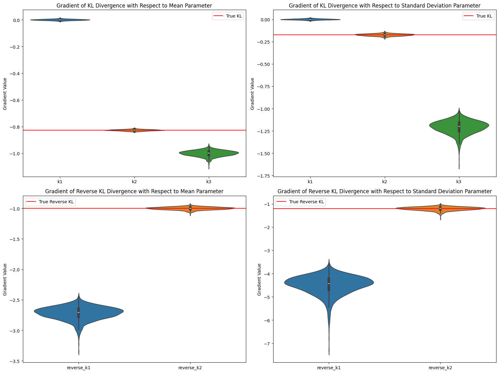
Fig. 2. Gradient Estimation of KL
Average gradient value comparison (mean parameter):
True KL gradient: -0.826446
k1 average gradient: 0.000137
k2 average gradient: -0.826291
k3 average gradient: -0.999618

Average gradient value comparison (standard deviation parameter):
True KL gradient: -0.173554
k1 average gradient: -0.000104
k2 average gradient: -0.173379
k3 average gradient: -1.209091

Reverse KL - Average gradient value comparison (mean parameter):
True Reverse KL gradient: -1.000000
reverse_k1 average gradient: -2.718389
reverse_k2 average gradient: -0.999755

Reverse KL - Average gradient value comparison (standard deviation parameter):
True Reverse KL gradient: -1.210000
reverse_k1 average gradient: -4.496196
reverse_k2 average gradient: -1.208987

KL - Comparison of bias and standard deviation for mean parameter gradients:
╒════╤═════════════╤══════════════╕
│    │   bias/true │   stdev/true │
╞════╪═════════════╪══════════════╡
│ k1 │      1.0002 │       0.0054 │
├────┼─────────────┼──────────────┤
│ k2 │      0.0002 │       0.0065 │
├────┼─────────────┼──────────────┤
│ k3 │      0.2095 │       0.026  │
╘════╧═════════════╧══════════════╛

KL - Comparison of bias and standard deviation for standard deviation parameter gradients:
╒════╤═════════════╤══════════════╕
│    │   bias/true │   stdev/true │
╞════╪═════════════╪══════════════╡
│ k1 │      0.9994 │       0.0359 │
├────┼─────────────┼──────────────┤
│ k2 │      0.001  │       0.0686 │
├────┼─────────────┼──────────────┤
│ k3 │      5.9667 │       0.4311 │
╘════╧═════════════╧══════════════╛

Reverse KL - Comparison of bias and standard deviation for mean parameter gradients:
╒════════════╤═════════════╤══════════════╕
│            │   bias/true │   stdev/true │
╞════════════╪═════════════╪══════════════╡
│ reverse_k1 │      1.7184 │       0.1081 │
├────────────┼─────────────┼──────────────┤
│ reverse_k2 │      0.0002 │       0.0231 │
╘════════════╧═════════════╧══════════════╛

Reverse KL - Comparison of bias and standard deviation for standard deviation parameter gradients:
╒════════════╤═════════════╤══════════════╕
│            │   bias/true │   stdev/true │
╞════════════╪═════════════╪══════════════╡
│ reverse_k1 │      2.7159 │       0.3419 │
├────────────┼─────────────┼──────────────┤
│ reverse_k2 │      0.0008 │       0.0636 │
╘════════════╧═════════════╧══════════════╛
Code
import torch
import numpy as np
import matplotlib.pyplot as plt
from torch.distributions import Normal
import seaborn as sns

# Set random seed for reproducibility
torch.manual_seed(42)
np.random.seed(42)

# Define parameters for two normal distributions
def setup_distributions(mu_theta=0.0, sigma_theta=1.0, mu_ref=1.0, sigma_ref=1.1):
    # Create trainable parameters
    mu_theta_param = torch.tensor(mu_theta, requires_grad=True)
    sigma_theta_param = torch.tensor(sigma_theta, requires_grad=True)

    # Reference distribution parameters (fixed)
    mu_ref_param = torch.tensor(mu_ref)
    sigma_ref_param = torch.tensor(sigma_ref)

    # Create distributions
    pi_theta = Normal(mu_theta_param, sigma_theta_param)
    pi_ref = Normal(mu_ref_param, sigma_ref_param)

    return pi_theta, pi_ref, mu_theta_param, sigma_theta_param

# Calculate the true KL divergence (analytical solution for normal distributions)
def true_kl_divergence(pi_theta, pi_ref):
    mu_theta = pi_theta.loc
    sigma_theta = pi_theta.scale
    mu_ref = pi_ref.loc
    sigma_ref = pi_ref.scale

    kl = (torch.log(sigma_ref/sigma_theta) +
          (sigma_theta**2 + (mu_theta - mu_ref)**2)/(2*sigma_ref**2) - 0.5)
    rkl = (torch.log(sigma_theta/sigma_ref) +
        (sigma_ref**2 + (mu_ref - mu_theta)**2)/(2*sigma_theta**2) - 0.5)

    return kl, rkl

# Three different KL divergence estimates
def k1_loss(x, pi_theta, pi_ref):
    return pi_theta.log_prob(x) - pi_ref.log_prob(x)

def k2_loss(x, pi_theta, pi_ref):
    return 0.5 * (pi_theta.log_prob(x) - pi_ref.log_prob(x))**2

def k3_loss(x, pi_theta, pi_ref):
    ratio = torch.exp(pi_ref.log_prob(x) - pi_theta.log_prob(x))
    return ratio - 1 - torch.log(ratio)

# Two different reverse KL divergence estimates
def reverse_k1_loss(x, pi_theta, pi_ref):
    ratio = torch.exp(pi_ref.log_prob(x) - pi_theta.log_prob(x))
    return ratio * (pi_ref.log_prob(x) - pi_theta.log_prob(x))

def reverse_k2_loss(x, pi_theta, pi_ref):
    return torch.exp(pi_ref.log_prob(x) - pi_theta.log_prob(x))

# Sample and compute gradients
def estimate_gradients(sample_size=10000, num_trials=10):
    pi_theta, pi_ref, mu_param, sigma_param = setup_distributions()

    # Compute the gradient of the true and reverse KL divergence
    true_kl, true_reverse_kl = true_kl_divergence(pi_theta, pi_ref)

    true_kl.backward()
    true_grad_mu = mu_param.grad.item()
    true_grad_sigma = sigma_param.grad.item()
    mu_param.grad.zero_()
    sigma_param.grad.zero_()

    true_reverse_kl.backward()
    true_reverse_grad_mu = mu_param.grad.item()
    true_reverse_grad_sigma = sigma_param.grad.item()
    mu_param.grad.zero_()
    sigma_param.grad.zero_()

    # Store gradients from different estimates
    k1_grads_mu = []
    k1_grads_sigma = []
    k2_grads_mu = []
    k2_grads_sigma = []
    k3_grads_mu = []
    k3_grads_sigma = []
    reverse_k1_grads_mu = []
    reverse_k1_grads_sigma = []
    reverse_k2_grads_mu = []
    reverse_k2_grads_sigma = []

    for _ in range(num_trials):
        pi_theta, pi_ref, mu_param, sigma_param = setup_distributions()

        # Sample from the current policy
        samples = pi_theta.sample((sample_size,))

        # Get gradient of KL estimation
        k1_values = k1_loss(samples, pi_theta, pi_ref)
        k1_mean = k1_values.mean()
        k1_mean.backward()
        k1_grads_mu.append(mu_param.grad.item())
        k1_grads_sigma.append(sigma_param.grad.item())
        mu_param.grad.zero_()
        sigma_param.grad.zero_()

        k2_values = k2_loss(samples, pi_theta, pi_ref)
        k2_mean = k2_values.mean()
        k2_mean.backward()
        k2_grads_mu.append(mu_param.grad.item())
        k2_grads_sigma.append(sigma_param.grad.item())
        mu_param.grad.zero_()
        sigma_param.grad.zero_()

        k3_values = k3_loss(samples, pi_theta, pi_ref)
        k3_mean = k3_values.mean()
        k3_mean.backward()
        k3_grads_mu.append(mu_param.grad.item())
        k3_grads_sigma.append(sigma_param.grad.item())
        mu_param.grad.zero_()
        sigma_param.grad.zero_()

        reverse_k1_values = reverse_k1_loss(samples, pi_theta, pi_ref)
        reverse_k1_mean = reverse_k1_values.mean()
        reverse_k1_mean.backward()
        reverse_k1_grads_mu.append(mu_param.grad.item())
        reverse_k1_grads_sigma.append(sigma_param.grad.item())
        mu_param.grad.zero_()
        sigma_param.grad.zero_()

        reverse_k2_values = reverse_k2_loss(samples, pi_theta, pi_ref)
        reverse_k2_mean = reverse_k2_values.mean()
        reverse_k2_mean.backward()
        reverse_k2_grads_mu.append(mu_param.grad.item())
        reverse_k2_grads_sigma.append(sigma_param.grad.item())
        mu_param.grad.zero_()
        sigma_param.grad.zero_()

    return {
        'true_grad_mu': true_grad_mu,
        'true_grad_sigma': true_grad_sigma,
        'k1_grads_mu': k1_grads_mu,
        'k1_grads_sigma': k1_grads_sigma,
        'k2_grads_mu': k2_grads_mu,
        'k2_grads_sigma': k2_grads_sigma,
        'k3_grads_mu': k3_grads_mu,
        'k3_grads_sigma': k3_grads_sigma,
        'true_reverse_grad_mu': true_reverse_grad_mu,
        'true_reverse_grad_sigma': true_reverse_grad_sigma,
        'reverse_k1_grads_mu': reverse_k1_grads_mu,
        'reverse_k1_grads_sigma': reverse_k1_grads_sigma,
        'reverse_k2_grads_mu': reverse_k2_grads_mu,
        'reverse_k2_grads_sigma': reverse_k2_grads_sigma
    }

def create_nice_table(results):
    true_grad_mu = results['true_grad_mu']
    true_grad_sigma = results['true_grad_sigma']
    true_reverse_grad_mu = results['true_reverse_grad_mu']
    true_reverse_grad_sigma = results['true_reverse_grad_sigma']
    k1_bias_mu = abs(np.mean(results['k1_grads_mu']) - true_grad_mu) / abs(true_grad_mu)
    k2_bias_mu = abs(np.mean(results['k2_grads_mu']) - true_grad_mu) / abs(true_grad_mu)
    k3_bias_mu = abs(np.mean(results['k3_grads_mu']) - true_grad_mu) / abs(true_grad_mu)
    k1_std_mu = np.std(results['k1_grads_mu']) / abs(true_grad_mu)
    k2_std_mu = np.std(results['k2_grads_mu']) / abs(true_grad_mu)
    k3_std_mu = np.std(results['k3_grads_mu']) / abs(true_grad_mu)
    k1_bias_sigma = abs(np.mean(results['k1_grads_sigma']) - true_grad_sigma) / abs(true_grad_sigma)
    k2_bias_sigma = abs(np.mean(results['k2_grads_sigma']) - true_grad_sigma) / abs(true_grad_sigma)
    k3_bias_sigma = abs(np.mean(results['k3_grads_sigma']) - true_grad_sigma) / abs(true_grad_sigma)
    k1_std_sigma = np.std(results['k1_grads_sigma']) / abs(true_grad_sigma)
    k2_std_sigma = np.std(results['k2_grads_sigma']) / abs(true_grad_sigma)
    k3_std_sigma = np.std(results['k3_grads_sigma']) / abs(true_grad_sigma)
    reverse_k1_bias_mu = abs(np.mean(results['reverse_k1_grads_mu']) - true_reverse_grad_mu) / abs(true_reverse_grad_mu)
    reverse_k2_bias_mu = abs(np.mean(results['reverse_k2_grads_mu']) - true_reverse_grad_mu) / abs(true_reverse_grad_mu)
    reverse_k1_std_mu = np.std(results['reverse_k1_grads_mu']) / abs(true_reverse_grad_mu)
    reverse_k2_std_mu = np.std(results['reverse_k2_grads_mu']) / abs(true_reverse_grad_mu)
    reverse_k1_bias_sigma = abs(np.mean(results['reverse_k1_grads_sigma']) - true_reverse_grad_sigma) / abs(true_reverse_grad_sigma)
    reverse_k2_bias_sigma = abs(np.mean(results['reverse_k2_grads_sigma']) - true_reverse_grad_sigma) / abs(true_reverse_grad_sigma)
    reverse_k1_std_sigma = np.std(results['reverse_k1_grads_sigma']) / abs(true_reverse_grad_sigma)
    reverse_k2_std_sigma = np.std(results['reverse_k2_grads_sigma']) / abs(true_reverse_grad_sigma)

    # Create table
    from tabulate import tabulate
    import pandas as pd

    df_mu = pd.DataFrame({
        'bias/true': [k1_bias_mu, k2_bias_mu, k3_bias_mu],
        'stdev/true': [k1_std_mu, k2_std_mu, k3_std_mu]
    }, index=['k1', 'k2', 'k3'])
    df_reverse_mu = pd.DataFrame({
        'bias/true': [reverse_k1_bias_mu, reverse_k2_bias_mu],
        'stdev/true': [reverse_k1_std_mu, reverse_k2_std_mu]
    }, index=['reverse_k1', 'reverse_k2'])
    df_sigma = pd.DataFrame({
        'bias/true': [k1_bias_sigma, k2_bias_sigma, k3_bias_sigma],
        'stdev/true': [k1_std_sigma, k2_std_sigma, k3_std_sigma]
    }, index=['k1', 'k2', 'k3'])

    df_reverse_sigma = pd.DataFrame({
        'bias/true': [reverse_k1_bias_sigma, reverse_k2_bias_sigma],
        'stdev/true': [reverse_k1_std_sigma, reverse_k2_std_sigma]
    }, index=['reverse_k1', 'reverse_k2'])

    # Format values
    df_mu = df_mu.round(4)
    df_sigma = df_sigma.round(4)
    df_reverse_mu = df_reverse_mu.round(4)
    df_reverse_sigma = df_reverse_sigma.round(4)

    # Print nice table
    print("KL - Comparison of bias and standard deviation for mean parameter gradients:")
    print(tabulate(df_mu, headers='keys', tablefmt='fancy_grid'))

    print("\nKL - Comparison of bias and standard deviation for standard deviation parameter gradients:")
    print(tabulate(df_sigma, headers='keys', tablefmt='fancy_grid'))

    print("\nReverse KL - Comparison of bias and standard deviation for mean parameter gradients:")
    print(tabulate(df_reverse_mu, headers='keys', tablefmt='fancy_grid'))

    print("\nReverse KL - Comparison of bias and standard deviation for standard deviation parameter gradients:")
    print(tabulate(df_reverse_sigma, headers='keys', tablefmt='fancy_grid'))

    return df_mu, df_sigma, df_reverse_mu, df_reverse_sigma


def visualize_results(results):
    fig, axes = plt.subplots(2, 2, figsize=(16, 12))

    axes[0,0].axhline(y=results['true_grad_mu'], color='r', linestyle='-', label='True KL')
    sns.violinplot(data=[results['k1_grads_mu'], results['k2_grads_mu'], results['k3_grads_mu']], ax=axes[0,0])
    axes[0,0].set_title('Gradient of KL Divergence with Respect to Mean Parameter')
    axes[0,0].set_xticks([0,1,2])
    axes[0,0].set_xticklabels(['k1', 'k2', 'k3'])
    axes[0,0].set_ylabel('Gradient Value')
    axes[0,0].legend()

    axes[0,1].axhline(y=results['true_grad_sigma'], color='r', linestyle='-', label='True KL')
    sns.violinplot(data=[results['k1_grads_sigma'], results['k2_grads_sigma'], results['k3_grads_sigma']], ax=axes[0,1])
    axes[0,1].set_title('Gradient of KL Divergence with Respect to Standard Deviation Parameter')
    axes[0,1].set_xticks([0,1,2])
    axes[0,1].set_xticklabels(['k1', 'k2', 'k3'])
    axes[0,1].set_ylabel('Gradient Value')
    axes[0,1].legend()

    axes[1,0].axhline(y=results['true_reverse_grad_mu'], color='r', linestyle='-', label='True Reverse KL')
    sns.violinplot(data=[results['reverse_k1_grads_mu'], results['reverse_k2_grads_mu']], ax=axes[1,0])
    axes[1,0].set_title('Gradient of Reverse KL Divergence with Respect to Mean Parameter')
    axes[1,0].set_xticks([0,1])
    axes[1,0].set_xticklabels(['reverse_k1', 'reverse_k2'])
    axes[1,0].set_ylabel('Gradient Value')
    axes[1,0].legend()

    axes[1,1].axhline(y=results['true_reverse_grad_sigma'], color='r', linestyle='-', label='True Reverse KL')
    sns.violinplot(data=[results['reverse_k1_grads_sigma'], results['reverse_k2_grads_sigma']], ax=axes[1,1])
    axes[1,1].set_title('Gradient of Reverse KL Divergence with Respect to Standard Deviation Parameter')
    axes[1,1].set_xticks([0,1])
    axes[1,1].set_xticklabels(['reverse_k1', 'reverse_k2'])
    axes[1,1].set_ylabel('Gradient Value')
    axes[1,1].legend()

    plt.tight_layout()
    plt.show()

    # Print mean comparison
    print("Average gradient value comparison (mean parameter):")
    print(f"True KL gradient: {results['true_grad_mu']:.6f}")
    print(f"k1 average gradient: {np.mean(results['k1_grads_mu']):.6f}")
    print(f"k2 average gradient: {np.mean(results['k2_grads_mu']):.6f}")
    print(f"k3 average gradient: {np.mean(results['k3_grads_mu']):.6f}")

    print("\nAverage gradient value comparison (standard deviation parameter):")
    print(f"True KL gradient: {results['true_grad_sigma']:.6f}")
    print(f"k1 average gradient: {np.mean(results['k1_grads_sigma']):.6f}")
    print(f"k2 average gradient: {np.mean(results['k2_grads_sigma']):.6f}")
    print(f"k3 average gradient: {np.mean(results['k3_grads_sigma']):.6f}")

    print("\nReverse KL - Average gradient value comparison (mean parameter):")
    print(f"True Reverse KL gradient: {results['true_reverse_grad_mu']:.6f}")
    print(f"reverse_k1 average gradient: {np.mean(results['reverse_k1_grads_mu']):.6f}")
    print(f"reverse_k2 average gradient: {np.mean(results['reverse_k2_grads_mu']):.6f}")

    print("\nReverse KL - Average gradient value comparison (standard deviation parameter):")
    print(f"True Reverse KL gradient: {results['true_reverse_grad_sigma']:.6f}")
    print(f"reverse_k1 average gradient: {np.mean(results['reverse_k1_grads_sigma']):.6f}")
    print(f"reverse_k2 average gradient: {np.mean(results['reverse_k2_grads_sigma']):.6f}")

    # Add nice table output
    print()
    df = create_nice_table(results)

if __name__ == "__main__":
    sample_size = 50000
    num_trials = 1000
    results = estimate_gradients(sample_size, num_trials)
    visualize_results(results)
Additional Notes
The variance reduction approach for k2 loss can follow Schulman (2020)’s analysis by introducing a zero-mean statistic and solving with the method of undetermined coefficients.
First, solve for $\theta$ component-wise:
$$ \begin{align*} \lambda_i^* &= \argmin_\lambda E_{X\sim\pi_\theta}\left[(\nabla_{\theta_i}\log\pi_{\theta}(X))^2 \cdot \left(\log\left(\frac{\pi_\theta(X)}{\pi_{ref}(X)}\right) - \lambda\right)^2\right]\\ &= \frac{E_{\pi_\theta}\left[(\nabla_{\theta_i}\log\pi_{\theta}(X))^2\cdot \left(\log\left(\frac{\pi_\theta(X)}{\pi_{ref}(X)}\right)\right)^2\right]}{E_{\pi_\theta}\left[(\nabla_{\theta_i}\log\pi_{\theta}(X))^2\right]}. \end{align*} $$
Then apply the modified estimator component-wise,
$$ \nabla_{\theta_i} = \nabla_{\theta_i} \frac{1}{2}(\log\pi_\theta(X) - \log\pi_{ref}(X) - \lambda_i^*)^2. $$
However, this approach is quite complicated. First, $\lambda$ is difficult to estimate as it requires computing the score (log prob gradient) first, potentially necessitating two backward passes. Second, each component needs to be estimated separately.
As an alternative, we could consider using the previous step’s score and a single $\lambda$ estimator:
$$ \hat{\lambda}^* = \frac{\sum_i|\nabla_{\theta_{old}}\log\pi_{\theta}(X_i)|_2^2\cdot \left(\log\left(\frac{\pi_\theta(X_i)}{\pi_{ref}(X_i)}\right)\right)^2}{\sum_i|\nabla_{\theta_{old}}\log\pi_{\theta}(X_i)|_2^2}. $$
However, this remains complex as it requires per-sample gradient norms and introduces some bias, which may not be worth the effort. The effectiveness of KL loss itself is uncertain, and whether additional variance reduction is needed here is debatable - perhaps k2 is already sufficient.
Citation
Please cite this work as:
Yang, Xiaobo. (Mar 2025). Gradient Estimation of KL Divergence in Large Language Model Reinforcement Learning. Xiabo’s Blog.
https://xiaobo-yang.github.io/posts/kl_grad/.
Or in BibTeX format:
@article{yang2025klgradient,
    title = "Gradient Estimation of KL Divergence in Large Language Model Reinforcement Learning.",
    author = "Yang, Xiaobo",
    journal = "xiaobo-yang.github.io",
    year = "2025",
    month = "Mar",
    url = "https://xiaobo-yang.github.io/posts/kl_grad/"
}
References
[1] John Schulman “Approximating KL Divergence.” 2020.
[2] Guo et al. “DeepSeek-R1: Incentivizing Reasoning Capability in LLMs via Reinforcement Learning” 2025.